From Dayan's Successor Representation to BFM for Humanoid Robots: Decoupling Environment Dynamics and Task Reward

Abstract

In 1993, Peter Dayan wrote in a paper: "Representation is the key—view a problem in the right way and it becomes easy." The "right way" he proposed was this: represent a state not by what it looks like, but by which states the agent will visit next. This idea, known as the Successor Representation (SR), launched a research program spanning three decades. In 2025, the product of that program—BFM-Zero, a single neural network with 440 million parameters—was deployed on a real Unitree G1 humanoid robot and, without any task-specific training, achieved motion tracking, goal reaching, and reward optimization in a zero-shot setting, even recovering on its own after being kicked over and continuing its task.

This article traces the complete intellectual lineage from theory to deployment: from Dayan's tabular SR, to Barreto's successor features and generalized policy improvement, to Blier's measure-theoretic formalization, to Touati and Ollivier's forward-backward (FB) representation, to Cetin's FB-AWARE (which made FB match single-task SOTA on offline RL benchmarks), to Tirinzoni's FB-CPR and Li's BFM-Zero (real humanoid robot deployment). We also cover two new directions from 2025–2026: Sikchi et al.'s ReLA/LoLA—fast adaptation in the BFM latent space that improves zero-shot policies by 10–40%; and Jajoo et al.'s RLDP—which replaces complex successor measure estimation with simple policy-agnostic latent dynamics prediction, showing distinctive robustness in low-coverage data scenarios.

This is not only one of the most complete theory-to-deployment stories in reinforcement learning; it also reveals an academic debate now taking shape: Does the future of BFM lie in increasingly sophisticated successor measure modeling, or in simpler, more robust alternatives?

---

1. Successor Representation — The Starting Point of Everything

Standard TD learning with function approximation has a hidden pitfall: generalization is determined by the metric of the representation, and this metric is usually spatial (Euclidean distance). When spatial proximity does not imply temporal proximity — for example, two rooms separated by a wall — generalization produces harmful interference.

Dayan's insight directly addressed this problem [Dayan1993]. He proposed that the representation of a state $i$ should not be its own coordinates or features, but rather the expected number of times it will visit all other states $j$ in the future under the current policy:

$$[{\overline{\mathbf{x}}}_i{]}_j=[\mathbf{I}{]}_{ij}+[\mathbf{Q}{]}_{ij}+[{\mathbf{Q}}^2{]}_{ij}+\cdots =[(\mathbf{I}-\mathbf{Q}{)}^{-1}{]}_{ij}$$

Here $\mathbf{Q}$ is the transition matrix. This successor representation captures the temporal proximity of states rather than spatial proximity — two states separated by a wall naturally become distant in the SR, because they can hardly reach each other.

The most elegant theoretical result of SR is this: under linear function approximation, learning the weights of the value function reduces to ${\mathbf{w}}^{\ast }=\mathbf{h}$ — only the immediate reward needs to be estimated. The entire temporal credit assignment problem is absorbed by the representation itself. In Dayan's words, TD methods become "a direct estimation problem, for which TD methods themselves are no longer necessary."

Even more forward-looking, Dayan raised two observations that would run through the following three decades of research: (1) a useful SR can be constructed during a "latent learning" phase before rewards appear — this anticipated later unsupervised RL; (2) when the policy changes during control, the SR degrades — a non-stationarity problem that remains not fully solved to this day.

Dayan validated these ideas on a $11\times 11$ grid world (Figure 1.1). After the agent explored the maze, the SR predictions starting from position (5,6) (Figure 1.2) exhibited a spatially ordered exponential decay — but note that the SR automatically "recognized" the obstacles: the predicted values for states on the far side of obstacles were almost zero, because they are spatially close yet temporally unreachable. This is precisely the core advantage of SR: what it represents is not spatial distance, but temporal distance. When the policy converged to the optimal path, the SR degenerated into predictions only along the path (Figure 4 in Dayan's paper), which Dayan called the "degeneration" of SR — a non-stationarity problem that still plagues all successor representation methods today.

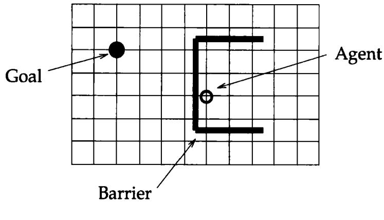
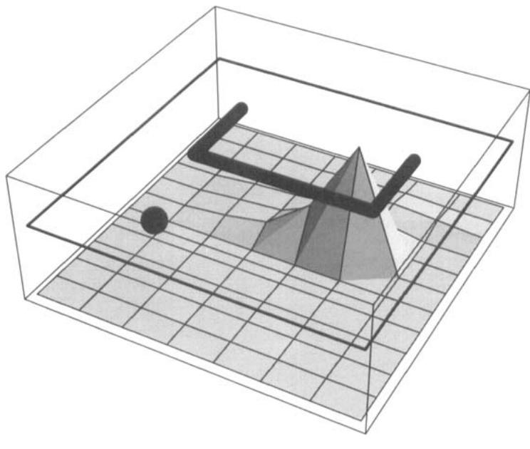
However, Dayan's SR was strictly limited to finite tabular MDPs. How to generalize it to continuous state spaces and use it for zero-shot task transfer became the key challenge of the next era.

---

2. From Representations to Transfer — Successor Features and GPI

Barreto et al. (2017) made two key generalizations [Barreto2017]:

First, they replaced the discrete indicator functions ${\mathbb{1}}_{\{s=j\}}$ with continuous feature mappings $\varphi (s,a,s^{\prime })\in {\mathbb{R}}^d$ . Successor Features (SFs) are defined as:

$${\psi }^{\pi }(s,a)={\mathbb{E}}^{\pi }[\sum _{i=t}^{\mathrm{\infty }}{\gamma }^{i-t}{\varphi }_{i+1}\mid S_t=s,A_t=a]$$

Under the assumption that rewards are linear in the features ( $r={\varphi }^{\mathrm{\top }}\mathbf{w}$ ), the value function decomposes into $Q^{\pi }(s,a)={\psi }^{\pi }(s,a{)}^{\mathrm{\top }}\mathbf{w}$ — dynamics and rewards are fully decoupled.

Second, and most critically: the Generalized Policy Improvement (GPI) theorem. Given a set of learned policies $\{{\pi }_i\}$ and their successor features, for a new task ${\mathbf{w}}^{\prime }$ , the GPI policy is:

$$\pi (s)=\arg \underset{a}{max}\underset{i}{max}{\tilde{\psi }}^{{\pi }_i}(s,a{)}^{\mathrm{\top }}{\mathbf{w}}^{\prime }$$

Barreto et al. proved that the performance lower bound of the GPI policy is the best individual policy's performance minus an approximation error term — and this guarantee holds even before the agent has taken any action on the new task. This effectively reframes transfer learning as an extension of dynamic programming: the Bellman optimality principle improves policies through maximization over a single policy, while GPI achieves policy improvement through maximization over multiple policies.

Barreto et al. (2017) validated SF&GPI on a four-room navigation task (Figure 2.1). The environment contains three types of objects (with different rewards), the goal is in a distant room, and task rewards are randomly resampled every 20,000 steps. The experimental results in Figure 2.2 show that all SFQL variants significantly outperform QL and PRQL — average return improves by more than 100%. More importantly, improvements on training tasks automatically generalize to untrained test tasks, even though the agent has never taken any action on those tasks. This generalization capability is precisely the core guarantee of the GPI theorem.

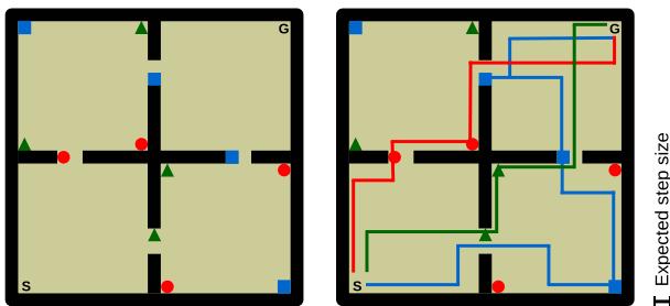
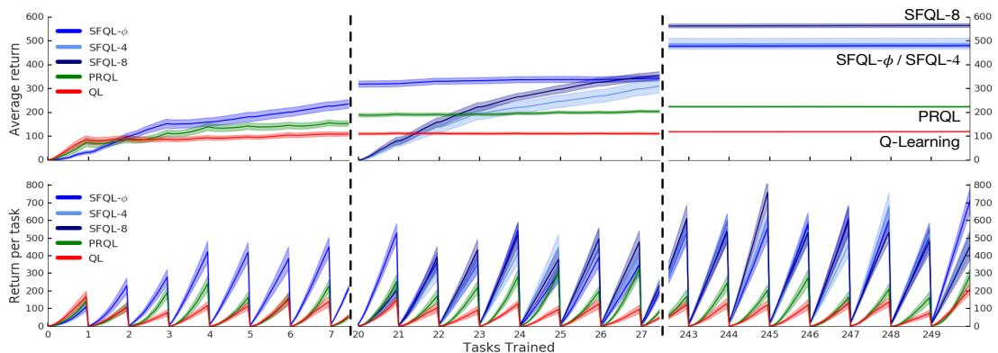
Borsa et al. (2018) further unified this framework [Borsa2018]. They proposed the Universal Successor Features Approximator (USFA): $\psi (s,a,\mathbf{z})$ is conditioned on both the task $\mathbf{w}$ and the policy $\mathbf{z}$ simultaneously. By varying the candidate set $\mathcal{C}$ , USFA interpolates continuously between two extremes: $\mathcal{C}=\{{\mathbf{w}}^{\prime }\}$ degenerates into UVFA (pure parametric generalization), and $\mathcal{C}=\mathcal{M}$ degenerates into SF&GPI (pure structural transfer). Borsa's performance bound reveals the core trade-off in choosing $\mathcal{C}$ : adding more policies can reduce the task distance ${\delta }_d$ , but simultaneously increases the risk of approximation error ${\delta }_{\psi }$ .

The success of the SF framework also exposed its fundamental limitation: everything depends on the choice of features $\varphi$ . But where do good features come from? Answering this question requires a deeper mathematical examination.

---

3. Completing the Mathematical Theory—The Successor State as a Linear Operator

Blier et al. (2021) provided a mathematical foundation for this problem by generalizing SR to general state spaces using measure theory [Blier2021]. They define the successor state operator:

$$M=(\mathrm{Id}-\gamma P{)}^{-1}=\sum _{n\ge 0}{\gamma }^n{P}^n$$

$M$ maps any reward function $R$ to a value function $V=MR$ —this is a linear operator. Within this framework, Blier et al. revealed three algebraic structures that go beyond the standard forward Bellman equation:

Backward Bellman equation: $M=\mathrm{Id}+\gamma MP$ . This is unique to the successor state—the value function has no counterpart. Its intuitive meaning is: add the observed transition to the "back" rather than the "front" of known paths. Mixing forward and backward TD reduces the multiplicity of the worst-converging eigenvalue from $n$ (the number of states) to $1$ .

Bellman-Newton operator: $M\leftarrow 2M-M(\mathrm{Id}-\gamma P)M$ . This is a second-order method corresponding to path concatenation—it doubles the length of known paths, whereas TD adds only one step at a time. Its continuous-time convergence rate is independent of the environment's eigenvalues, unlike TD, which is limited by the spectral gap $1-\gamma$ .

Forward-backward (FB) decomposition: $M(s_1,s_2)\approx F(s_1{)}^{\mathrm{\top }}B(s_2)$ . Blier et al. proved that the fixed point of the FB variant fb-FB corresponds to the truncated SVD of $M$ , focusing on low-frequency, long-range dependencies. This provides a solid theoretical foundation for FB representations—it is not an ad hoc engineering trick, but rather the natural low-rank structure of the successor state operator.

Figure 3.1 compares these three mechanisms intuitively from a path perspective. Given an observed transition $s\to s^{\prime }$ , forward TD adds it to the front of all known paths—suitable for reasoning with a fixed goal state; backward TD adds it to the back—suitable for reasoning with a fixed starting point. Bellman-Newton, by contrast, performs path concatenation: it connects all paths to $s$ , the transition $s\to s^{\prime }$ , and all paths departing from $s^{\prime }$ , roughly doubling the length of known paths. In continuous time, the convergence rate of this operation is independent of the environment's eigenvalues—unlike TD, which is limited by the spectral gap $1-\gamma$ . Blier et al. proved that the fixed point of fb-FB corresponds to the truncated SVD of $M$ , meaning that FB automatically focuses on long-range, low-frequency structure in the environment, making it naturally suited to capturing macroscopic patterns in reward functions.

Blier's FB decomposition was derived for a fixed policy. Touati and Ollivier's breakthrough lay in realizing that if the policy itself is made to depend on the same latent variable $z$ , FB can go much further.

---

4. The FB Algorithm—Learn One Representation, Optimize All Rewards

Touati and Ollivier (2021) posed a bold question [Touati2021]: can one learn, purely from environment interaction and without any reward signal, a compact object from which the optimal policy for any reward function specified after the fact can be read off directly—with no planning at all?

FB's answer is to learn two functions $F(s,a,z)$ and $B(s,a)$ such that $F^{\mathrm{\top }}B$ approximates the successor state density. The FB framework then operates in a closed loop of three steps:

1. Unsupervised learning phase: learn $F$ and $B$ from reward-agnostic environment interaction.
2. Reward encoding: for any reward function $r$ , compute $z_R={\mathbb{E}}_{(s,a)\sim \rho }[r(s,a)B(s,a)]$ —an expectation, a single forward pass.
3. Optimal policy extraction: directly use ${\pi }_{z_R}(s)=\arg \underset{a}{max}F(s,a,z_R{)}^{\mathrm{\top }}{z}_R$ —no planning, no gradient descent, no fine-tuning.

This is the core of the FB paradigm: $B$ is a universal reward encoder, mapping any reward function to a $d$ -dimensional vector; $F$ is a universal policy decoder, outputting the corresponding optimal policy given any $z$ . Theorem 1 gives an optimality guarantee under perfect training; Theorem 5 proves that under approximate training, the suboptimality is proportional to the model's approximation error ( $\frac{3\epsilon \parallel r{\parallel }_{\mathrm{\infty }}}{1-\gamma }$ ).

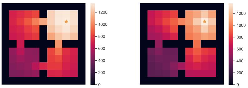
An important property of FB is illustrated intuitively in Figure 4.1: the representation rank $d$ controls spatial precision. When $d=25$ , the estimated optimal Q-values become "blurred" near the target—the agent often stops beside the target rather than reaching it precisely. When $d=75$ , the Q-value heatmap at the target location is sharply focused, and the agent reaches the target precisely. This reveals FB's core trade-off: too small a $d$ leads to reward blurring—a low-rank approximation amounts to keeping only the first $d$ principal components of the successor measure, discarding fine-grained spatial information. Blier2021 explains this theoretically: FB corresponds to a truncated SVD of $M$ , and a small $d$ captures only the lowest-frequency, longest-range dynamics modes.

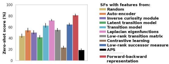
Touati et al. (2023) subsequently provided a systematic empirical verdict [Touati2023]. Across 4 environments, 13 tasks, and 3 different exploration buffers (RND, APS, Proto), each with 10 random seeds (Figure 4.2): FB reached 81% of supervised offline TD3 performance (best case 85% with the RND buffer), significantly outperforming the best SF variant (Laplacian eigenfunctions, 74%). The box plots in Touati's paper further reveal variance differences across methods—FB not only has the highest average performance, but also the best stability across environments and buffers. The core finding is that most feature-learning methods produce features with effective rank collapse—in maze-like environments, only about 30% of eigenvalues exceed the threshold, whereas FB features have a much more uniform spectral distribution.

However, these results all come from mazes, Pac-Man, and simple locomotion tasks. For FB to become practical, two key bottlenecks must still be addressed: (1) on standard offline RL benchmarks (such as D4RL), native FB performance is nearly zero—its TD3-style policy optimization suffers severe distribution shift on datasets with narrow behavior distributions; (2) FB's task encoding $z=\mathbb{E}[rB]$ is linear, limiting the spatial precision and expressive power of the task representation. Cetin et al. (2024)'s FB-AWARE addresses both problems simultaneously [Cetin2024].

---

5. Making FB Practical — FB-AWARE's Offline RL and Autoregressive Features

The challenge of offline RL: from zero to matching SOTA. Native FB scores only 22.3 in total on D4RL locomotion-v2, while the single-task SOTA method XQL reaches 752.9 — a gap of more than 30x. The problem is that FB's native TD3 policy improvement produces catastrophic extrapolation errors on offline data.

FB-AWARE's solution has two parts. First, Advantage-Weighted Regression (AW): replace TD3-style policy improvement with weighted behavior cloning — actions in the dataset are weighted by exponentiated advantages, using improved weighted importance sampling (IWIS) to reduce the bias from $O(n^{-1})$ to $O(n^{-2})$ . Combined with evaluation-based sampling (sample $M$ actions from the policy, execute the one with the highest $Q$ value) and dual F-network uncertainty representation (using the mean rather than taking the minimum), FB-AW achieves the critical leap from zero to satisfactory performance on difficult environments such as Humanoid.

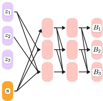
Autoregressive features: breaking the linear constraint. FB's second limitation stems from its task encoding scheme. In native FB, $z=\mathbb{E}[r(s)B(s)]$ is a linear function of $r$ — a task is identified as a vector of correlations with a fixed set of features $B$ . Cetin et al. propose autoregressive features: decompose $z$ and $B$ into $K$ blocks, computed hierarchically:

$$z_1=\mathbb{E}[r(s)B_1(s)],z_2=\mathbb{E}[r(s)B_2(s,z_1)],z_3=\mathbb{E}[r(s)B_3(s,z_1,z_2)],\dots$$

Later feature blocks are conditioned on earlier task encodings, allowing the overall task representation $r\mapsto z$ to be an arbitrary nonlinear mapping (Appendix Theorem A.3 proves that a two-layer autoregressive structure achieves universal approximation). Intuitively, $z_1$ provides coarse-grained task localization ("the reward is in the upper-left corner"), and $z_2$ uses this information to extract finer features. In implementation, this is efficiently realized with a masked MLP — the connections from $z_i$ to output block $B_j$ ( $j\le i$ ) are removed.

Experimental results. On D4RL locomotion-v2, FB-AWARE scores 719.5 in total, significantly narrowing the gap with reward-trained single-task SOTA methods (XQL: 752.9, IQL: 692.6) — while FB-AWARE is always a reward-free, zero-shot generalist agent. The table below shows the full comparison on D4RL (excerpted from Cetin2024 Table 1):

Dataset	BC	IQL	XQL	FB (native)	FB-AW	FB-AWARE
halfcheetah-medium	42.6	47.4	48.3	49.0	60.0	62.7
hopper-medium	52.9	66.3	74.2	0.9	59.1	59.9
walker2d-medium	75.3	78.3	84.2	0.5	80.5	89.6
halfcheetah-med-replay	36.6	44.2	45.2	30.8	52.7	50.8
hopper-med-replay	18.1	94.7	100.7	16.4	87.1	89.6
walker2d-med-replay	26.0	73.9	82.2	9.9	91.7	98.8
halfcheetah-med-expert	55.2	86.7	94.2	91.7	99.6	100.1
Locomotion-v2 total	466.7	692.6	752.9	22.3	696.2	719.5

Native FB scores only 22.3 in total (nearly zero on hopper-medium), while FB-AWARE's 719.5 approaches reward-trained XQL (752.9) — demonstrating the necessity of offline RL techniques for BFM training. On the Jaco arm goal-reaching task, autoregressive features yield roughly a 15% relative improvement. On FrankaKitchen, FB-AWARE (52.5/53.5) is comparable to IQL (46.3/51.0).

Figure 5.1 illustrates the implementation of the autoregressive $B$ network: connections in each layer are masked so that low-index output blocks can only see high-index input blocks. This is a hierarchical prior — encouraging coarse-grained features ( $B_1$ ) to first localize the macroscopic region of the task, and fine-grained features ( $B_2,B_3,\dots$ ) to then extract precise details given the region information. At test time, computing the fixed point requires multiple network forward passes (each block computed separately), but at training time the mask structure enables a single efficient forward pass.

On the Jaco arm goal-reaching task (Figure 5.2), FB-AW more than doubles native FB's performance, and FB-AWARE (4 autoregressive blocks) adds roughly another 15% on top. Notably, the advantage of autoregressive features is most pronounced when the representation dimension $d$ is small — consistent with intuition: when total dimensionality is constrained, hierarchically reusing representational capacity is more efficient than allocating it uniformly. Figures 3 and 4 in Cetin et al. show evaluation results on in-dataset and out-of-dataset tasks on DMC locomotion tasks respectively: the AW component is decisive on Humanoid (near-zero performance without AW), while autoregressive features provide small but systematic gains on out-of-dataset tasks.

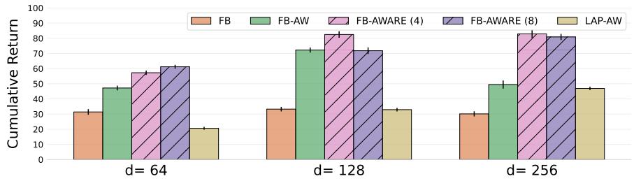
An intriguing finding: although autoregressive features theoretically extend FB's expressiveness from a linear subspace to arbitrary nonlinear manifolds, the gains in most experiments are modest. Cetin et al. speculate that BFM expressiveness may not be the primary bottleneck on current benchmarks — data quality and offline optimization techniques are the decisive factors.

Toward humanoid robots. FB-AWARE demonstrates that a general-purpose, reward-free FB BFM can match single-task SOTA methods on standard offline RL benchmarks. The next question is: can FB scale to 69-dimensional action spaces and unstable whole-body humanoid robot control?

6. Behavior Foundation Models — FB for Controlling Real Robots

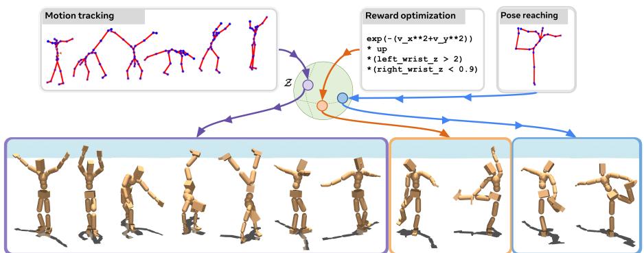
Tirinzoni et al. (2025) answered this with FB-CPR [Tirinzoni2025]. The core challenge is that unsupervised FB exploration in a 69-dimensional action space produces useless, unstable behaviors. The solution is Conditional Policy Regularization (CPR): embed unlabeled motion capture trajectories into a latent space ( $z_{\tau }=\frac{1}{|\tau |}\sum _{s\in \tau }B(s)$ ), then train a GAN discriminator $D(s,z)$ conditioned on $z$ to distinguish the dataset distribution from the policy distribution. The actor maximizes a combined objective:

$${\mathcal{L}}_{\mathrm{FB}-\mathrm{CPR}}(\pi )=-\mathbb{E}[F(s,a,z{)}^{\mathrm{\top }}z+\alpha Q_D(s,a,z)]$$

where $Q_D$ is the value function of the discriminator log-ratio reward. The result: FB-CPR achieves on average 73.4% of the performance of single-task upper-bound algorithms across three categories — reward optimization, goal reaching, and motion tracking — all zero-shot. Human evaluators judged FB-CPR's motions as more natural than pure TD3 in 83% of reward tasks and 69% of goal tasks. After scaling the model to 288 million parameters, all metrics improved monotonically.

The FB-IL overview by Pirotta et al. (2024) is shown in Figure 6.1. The core idea is simple yet powerful: all mainstream imitation learning principles can be expressed as the problem of optimizing $z$ in the latent space $\mathcal{Z}$ — behavior cloning (BC) minimizes the action distribution divergence between expert and policy, distribution matching (DM) minimizes the divergence in state visitation distributions, and Bellman residual methods minimize the Bellman error between the expert successor measure and the policy successor measure. Because $z$ has only 50–100 dimensions (whereas the policy network has millions of parameters), optimization can be completed in seconds — FB-IL reaches 80–95% of expert performance in 5 seconds, while the offline IL baseline DEMODICE requires nearly 13 hours — a three-order-of-magnitude speedup.

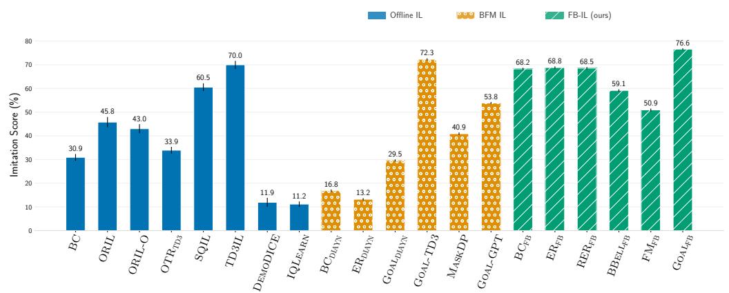
Pirotta et al. (2024) demonstrated another dimension of FB [Pirotta2024]: the same pre-trained FB model can be used for instant imitation learning. Given a small number of expert trajectories, different IL principles — behavior cloning, distribution matching, Bellman residual minimization — all reduce to optimizing $z$ in a low-dimensional latent space ( $d=50$ – $100$ ), rather than fine-tuning the entire policy network. ${\mathrm{ER}}_{\mathrm{FB}}$ reaches 80–95% of expert performance in under 5 seconds; even the most complex Bellman residual method takes only about 4 minutes, while offline IL baselines (such as DEMODICE) require nearly 13 hours — a three-order-of-magnitude speedup.

The core architecture of FB-CPR is shown in Figure 6.2. Unlabeled motion capture trajectories are embedded into a latent space via the $B$ network to obtain $z_{\tau }$ , and then a GAN discriminator $D(s,z)$ learns to distinguish "real" (dataset state, $z$ ) pairs from "fake" (policy-generated state, $z$ ) pairs. The log-ratio of this discriminator constitutes an intrinsic reward signal that guides the policy to produce natural, human-like motions while optimizing task objectives — without any explicit motion labels.

Li et al. (2025)'s BFM-Zero is the current endpoint of this arc [Li2025]: deploying FB-CPR from simulation to a real Unitree G1 humanoid robot. Three key sim-to-real extensions: (1) asymmetric training — the Actor receives noisy observation history, while the Critic accesses privileged simulation states; (2) large-scale domain randomization (mass, friction, joint offsets, center-of-mass offsets); (3) an auxiliary safety Critic (joint limits, self-collision, foot slip). Figure 6.3 shows the complete BFM-Zero pipeline from simulation to reality. The three key sim-to-real extensions are highlighted in the figure — (1) asymmetric Actor-Critic architecture: the Actor receives only noisy observation history (simulating real sensors), while the Critic accesses privileged simulation states during training; (2) extensive domain randomization covering physical parameters such as mass, friction, and joint offsets; (3) an auxiliary safety Critic providing penalty signals for joint limits, self-collision, and foot slip. These design choices enable a BFM trained in simulation to transfer zero-shot to real hardware, without any fine-tuning.

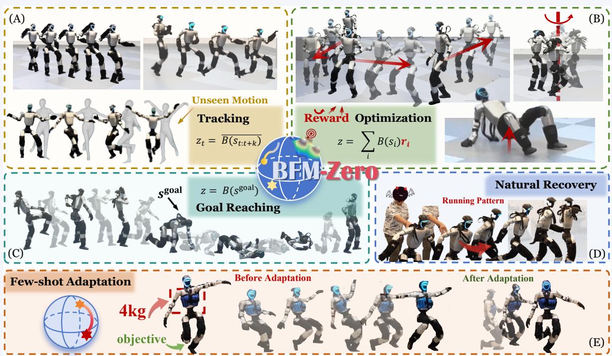
The most striking result is disturbance recovery: after being pushed, kicked, or even dragged to the ground, the robot naturally recovers and continues executing its task — this is not achieved through explicit robustness training, but because the structured skill repertoire in the FB latent space enables the policy to flexibly switch to alternative behavior modes. Under a 4 kg load, optimizing latent variables via the cross-entropy method (CEM) extended single-leg standing time from under 5 seconds to over 15 seconds, and reduced motion tracking error by 29.1%.

The success of these applications also gives us a clearer view of the boundaries of the current paradigm. But there remains a practical issue: even the best BFM produces suboptimal zero-shot policies — errors during inference (the linear projection of $z_r=\mathbb{E}[rB]$ ) cause performance loss. Sikchi et al. (2025) posed a direct question: can this gap be rapidly closed within a few online interactions [Sikchi2025]?

---

7. Rapid Adaptation — Mining Better Policies from the BFM Latent Space

Figure 7.1 summarizes the core intuition behind the method of Sikchi et al. Unsupervised pre-training of any BFM produces two things: (1) a policy space $\{{\pi }_z\}$ parameterized by a low-dimensional latent variable $z$ , and (2) an inference procedure $r\mapsto z_r$ that maps reward functions into the latent space. The zero-shot policy ${\pi }_{z_r}$ is the output of the inference procedure. The central finding of Sikchi et al. is that ${\pi }_{z_r}$ is not the best policy in $\{{\pi }_z\}$ — the bottleneck lies in the inference procedure (the linear projection $\mathbb{E}[rB]$ loses the fine-grained structure of the reward), not in the policy space itself. Their proposed ReLA and LoLA find significantly better $z$ by taking a small number of gradient steps in the latent space, without changing the policy network parameters.

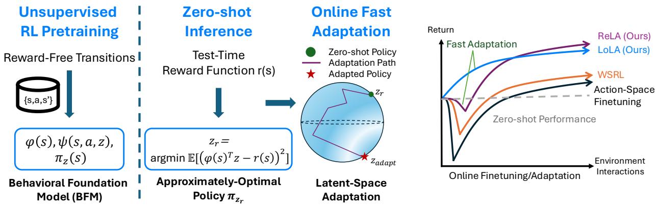
Key finding: the BFM latent space already contains policies better than zero-shot inference. Sikchi et al. show that in the latent policy spaces $\{{\pi }_z\}$ of four BFMs — FB, HILP, PSM, and FB-CPR — there exist policies whose performance significantly exceeds the zero-shot policy ${\pi }_{z_r}$ . The bottleneck is not the policy space, but the inference process.

Why search in the latent space? The latent variable $z$ has only about 100 dimensions, while the policy network has millions of parameters. Fine-tuning all parameters in action space (e.g., TD3-I) leads to catastrophic "forgetting" — performance drops sharply before recovering. Sikchi et al. propose two complementary algorithms for searching in the latent space:

ReLA (Residual Latent Adaptation): an off-policy actor-critic method. It decomposes the Q-function into a frozen BFM base term plus a learnable residual term:

$$Q_r^{{\pi }_z}(s,a)=\psi (s,a,z{)}^{\mathrm{\top }}{z}_r+Q^{\text{residual}}(s,a;\theta )$$

The residual critic only needs a small network (2-layer MLP, 64 hidden units vs. 1024 units for a full critic), because in theory it only needs to correct the reward projection error $(I-{\mathrm{\Pi }}_B)r$ . Gradients flow only through $z$ , and the policy network remains frozen. However, ReLA still suffers initial performance degradation in some environments — distribution shift during critic training causes "unlearning."

LoLA (Lookahead Latent Adaptation): a pure actor method that completely sidesteps the distribution shift problem of critic learning. It parameterizes a Gaussian distribution over latent variables ${\pi }_{\mu ,\sigma }=\mathcal{N}(\mu ,\sigma )$ , initialized from $\mu =z_r$ . It samples $k$ latent variables, performs $n$ steps of online rollout, and bootstraps terminal-state values using the frozen BFM successor features:

$$R^n(s_0,z)=\sum _{t=0}^{n-1}{\gamma }^{t}r(s_{t+1})+{\gamma }^n\psi (s_{n+1},{\pi }_z(s_{n+1}),z{)}^{\mathrm{\top }}{z}_r$$

It then estimates gradients using REINFORCE with a leave-one-out baseline. LoLA runs 157 times faster than ReLA (2,200 vs. 14 FPS) and achieves monotonic performance improvement — initial performance never drops, which holds across all BFMs and all tested domains.

Experimental results. Across 4 BFMs and 64 tasks, LoLA achieves 10–40% improvement within a few dozen episodes. On HumEnv (45 humanoid robot tasks), it improves by about 10% within 20 episodes and about 40% within 200 episodes. Cosine similarity analysis reveals an interesting phenomenon: ReLA drifts farther from $z_r$ in the latent space (correlated with performance fluctuations), while LoLA stays closer yet still finds significantly better policies — indicating that policies with similar performance may correspond to very different latent variables.

Figure 7.2 summarizes the aggregated performance improvement across all methods and BFMs (top) and the change in cosine similarity in the latent space (bottom). The vertical axis of the top plot is the percentage performance improvement relative to the zero-shot policy. It is clear that action-space fine-tuning methods (TD3-I, gray line) suffer a significant initial performance collapse on almost all BFMs — even falling below the zero-shot baseline. ReLA (blue) also shows a small drop in some domains (especially Pointmass), but far less severe than action-space methods. LoLA (green) achieves monotonic improvement on all BFMs and all tasks — the curve never falls below zero. The bottom plot explains why: ReLA drifts farther from $z_r$ in the latent space (cosine similarity drops quickly), while LoLA stays near $z_r$ and makes fine adjustments — the "small steps, fast iteration" strategy is more effective for latent-space search.

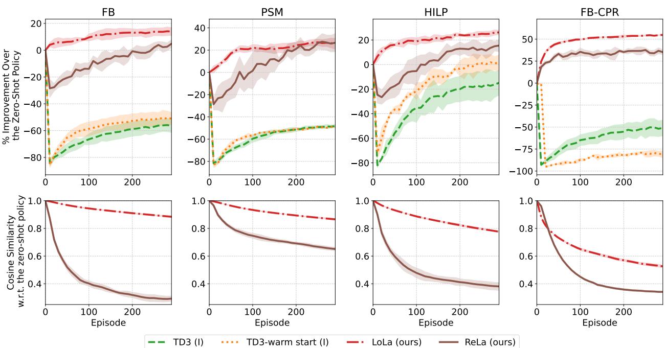
A practical takeaway: between LoLA and ReLA, LoLA's monotonic improvement and computational efficiency (157× ReLA's FPS) make it the default choice for practical deployment — provided that arbitrary state resets (privileged resets) are available. This further reinforces the finding of Pirotta2024: the structured nature of the BFM latent space makes searching within it far more efficient than fine-tuning the entire model.

8. A Simpler Path? — RLDP Challenges the FB Consensus

The core assumption of BFM is that good state representations must be obtained by learning successor measures. FB, PSM, and HILP all jointly optimize representations and successor features through Bellman backups — but this also introduces bootstrapping instability, the need to specify policy/reward classes a priori, and potentially extrapolated action queries. Jajoo et al. (2026) posed a challenging question [Jajoo2026]: are these complex representation-learning objectives really necessary for zero-shot RL?

RLDP (Regularized Latent Dynamics Prediction): a simple two-stage alternative.

Stage One — Representation Learning. Learn a state encoder $\varphi :\mathcal{S}\to {\mathbb{R}}^d$ by predicting future latent states — a fully policy-agnostic supervised learning objective:

$${\mathcal{L}}_d(\varphi ,g,w)={\mathbb{E}}_{\tau \sim \mathcal{D}}[\sum _{t=1}^H\parallel h_t-\overline{\varphi }(s_t){\parallel }^2],h_{t+1}=g(h_t,a_t{)}^{\mathrm{\top }}w$$

where $h_0=\varphi (s_0)$ , $\overline{\varphi }$ are slowly moving target encoders (EMA). Figure 8.1 illustrates RLDP's two-stage design. Stage one (representation learning) is completely independent of the policy — the encoder $\varphi$ is trained solely by predicting "what the future latent state will be, given the current state and an action sequence." This avoids all the problems of Bellman backups in FB/PSM/HILP: no need to specify policy or reward classes, no extrapolated action queries, no bootstrapping instability. Stage two (BFM training) freezes $\varphi$ and trains the successor features $\psi$ and policy ${\pi }_z$ with the standard successor measure contrastive loss — exactly the same as the second stage of methods like FB, except the representation no longer participates in gradient updates.

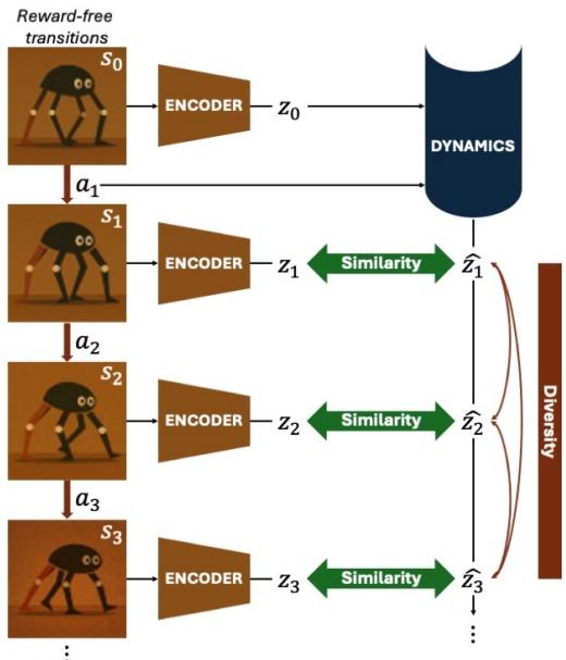
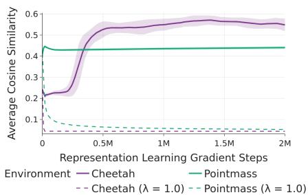
Jajoo et al. found that latent dynamics prediction alone leads to "mild feature collapse" — the cosine similarity of state representations increases with training, shrinking the span of representable reward functions. The solution is simple and effective: add orthonormal regularization:

$${\mathcal{L}}_r(\varphi )={\mathbb{E}}_{s,s^{\prime }\sim \rho }[\varphi (s{)}^{\mathrm{\top }}\varphi (s^{\prime })]$$

Project features onto the hypersphere ${\mathbb{S}}^{d-1}$ and minimize the cosine similarity of randomly sampled state pairs. Even with a very small regularization coefficient $\lambda =0.01$ , this is sufficient to maintain feature diversity.

Theoretical Foundation. Lemma 4.3 proves that minimizing the RLDP loss upper-bounds the successor measure prediction error for any Lipschitz value policy — providing a formal guarantee for why dynamics-prediction features are suitable for BFM training.

Stage Two — BFM Training. Freeze $\varphi$ and train the successor features $\psi (s,a,z)$ and policy ${\pi }_z$ with the standard successor measure contrastive loss. This is entirely a standard BFM — except the representation comes from policy-agnostic dynamics prediction rather than Bellman backups.

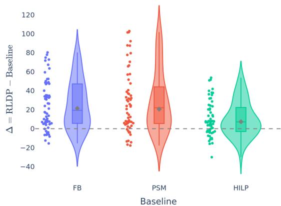
Experimental Results. On the standard DMC + ExoRL benchmarks, RLDP matches or surpasses FB, PSM, and HILP. On 45 SMPL humanoid robot tasks, RLDP is competitive with baseline methods, and on some tasks even exceeds oracle performance. But RLDP's real advantage lies in low-coverage data scenarios: on 6 tasks from the D4RL medium and medium-expert datasets, RLDP surpasses all baselines on 5 tasks — whereas Bellman-backup-based methods (FB, PSM, HILP) perform significantly worse in these low-coverage settings. The reason is RLDP's policy-agnosticism — it only uses the $(s,a,s^{\prime })$ transitions actually observed in the dataset and never queries extrapolated actions.

Figure 8.2 is the most diagnostic experimental result in the RLDP paper. It shows the change in average cosine similarity of randomly sampled state pairs during training — without regularization (blue), similarity rises monotonically from about 0.45 to 0.55+, indicating that all state representations are trending toward homogeneity. This "mild collapse" is not as thorough as full collapse (all representations collapsing to a single point) — the dynamics prediction loss is still decreasing — but it systematically shrinks the span of representable reward functions. Adding orthonormal regularization with $\lambda =1$ (orange) stably maintains similarity around 0.35 — feature diversity is preserved. Subsequent ablation studies (Figure 5 in Jajoo et al.) further confirm that even $\lambda =0.01$ yields statistically significant performance improvements.

RLDP's most striking results come from low-coverage data scenarios (Figure 8.3). On 6 tasks from the D4RL medium and medium-expert datasets, RLDP surpasses FB, PSM, and HILP on 5 tasks — each point represents the $\mathrm{\Delta }=R_{\text{RLDP}}-R_{\text{baseline}}$ for a (task, seed) pair. The IQM (interquartile mean) marked by gray diamonds is positive in all comparisons, with most of the mass distributed above the zero line. This is directly related to RLDP's policy-agnosticism: FB/PSM/HILP need to query extrapolated actions under the current policy when training representations — under a narrow data distribution, these extrapolated queries give severely wrong Q-value estimates, which in turn corrupt representation learning. RLDP only uses the $(s,a,s^{\prime })$ actually present in the data — no extrapolation, no contamination.

Paradigm Tension. RLDP's introduction sparked a fundamental methodological debate in the BFM field. The FB lineage holds that successor measure estimation is necessary; RLDP demonstrates that policy-agnostic latent dynamics prediction can match or even surpass these methods, especially in low-coverage data scenarios. However, RLDP has not yet been tested at the humanoid robot scale (69-dimensional action space) where FB-CPR has succeeded. Whether the two approaches can be combined — for example, replacing the jointly learned $B$ in FB with RLDP representations — is an open direction for exploration.

---

9. Open Problems and Future Directions

Fixed dynamics assumption: From Dayan1993 to Jajoo2026, all papers assume that environment transition dynamics are stationary [Dayan1993, Li2025]. In reality, dynamics change continuously—payload, terrain, wear. Sikchi2025's LoLA provides fast online adaptation, and Li2025's CEM reduces tracking error by 29.1% under payload variation—but these are reactive. A BFM that can predict or remain invariant to dynamics changes has yet to emerge.

The representation learning paradigm debate: The FB lineage holds that learning successor measures through Bellman backups is necessary [Touati2021, Cetin2024, Tirinzoni2025]. Jajoo2026's RLDP challenges this consensus—demonstrating that policy-agnostic latent dynamics prediction can match or even surpass these methods, with distinctive robustness especially in low-coverage data scenarios [Jajoo2026]. But RLDP has not yet been tested at the scale of humanoid robot control with 69-dimensional action spaces. Whether the two approaches can be combined—for example, initializing FB's $B$ network with RLDP representations—is an open empirical question.

The inference-versus-adaptation trade-off: Sikchi2025 proves that better policies do exist in the BFM latent space; zero-shot inference simply cannot find them [Sikchi2025]. Cetin2024's autoregressive features partially address this through nonlinear inference [Cetin2024]. But whether the optimal policy is more efficiently found at training time or test time remains unsettled.

Environment-specific pre-training: Every BFM must be trained from scratch for each new robot or environment [Tirinzoni2025, Li2025]. Jajoo2026's two-stage RLDP (representation→policy) hints at a partially decoupled direction: if representations can be shared across environments, only the policy needs retraining—but this has not yet been demonstrated.

The interaction between data quality and algorithms: Cetin2024's finding is intriguing: on high-quality MOOD data, advantage weighting is necessary; on low-quality RND exploration data, advantage weighting is actually harmful [Cetin2024]. Jajoo2026 further demonstrates that policy-agnostic representations are more robust in low-coverage scenarios [Jajoo2026]. But no work provides formal guiding principles for data collection in BFM pre-training.

Scaling laws: Li2025 reports that the scaling behavior of model and data size has not been systematically characterized. Tirinzoni2025 shows that 2× scaling yields monotonic improvement. Cetin2024 indicates that on current benchmarks, data quality matters more than model expressiveness [Cetin2024]. Whether FB-class BFMs obey predictable scaling laws like LLMs, and how data quality and model scale interact, remain principled open questions.

---

10. Conclusion

The successor representation can be said to be one of the most successful ideas in reinforcement learning—not because it was practical when first proposed (Dayan's 1993 paper only ran experiments on an 11×11 grid world), but because it identified a fundamental decomposition: dynamics can be separated from reward.

Each generation resolved the key limitation of the previous one: Dayan introduced SR but was restricted to tabular MDPs [Dayan1993]; Barreto generalized to continuous spaces but required hand-crafted features [Barreto2017]; Touati and Ollivier eliminated the feature bottleneck by jointly learning $F$ and $B$ [Touati2021]; Cetin used autoregressive features and advantage-weighted regression to make FB match single-task SOTA on offline RL benchmarks [Cetin2024]; Tirinzoni and Li extended FB to real humanoid robots [Tirinzoni2025, Li2025]; Sikchi et al. showed that searching in the BFM latent space can rapidly surpass zero-shot policies [Sikchi2025].

But 2025–2026 also brought a challenge: Jajoo et al.'s RLDP showed that simple policy-agnostic latent dynamics prediction can match or even surpass the complex successor measure machinery on which the entire FB lineage was built—especially in low-coverage scenarios where Bellman backups break down [Jajoo2026]. This constitutes a healthy academic tension within the field: does the future of BFM lie in increasingly sophisticated successor measure modeling, or in simpler, more robust alternatives?

If the methodology of the past three decades offers any lesson, it is this: the next breakthrough will come from seeing the problem in "the right way"—a way that, in hindsight, makes the difficulty look trivial. And whether that "right way" is successor measures, latent dynamics, or something not yet imagined, is the central question of the coming decade. As Dayan wrote in 1993: "Representation is the key."

References

• [Dayan1993] Dayan, P. (1993). Improving Generalization for Temporal Difference Learning: The Successor Representation. Neural Computation, 5(4), 613–624.
• [Barreto2017] Barreto, A., Dabney, W., Munos, R., Hunt, J. J., Schaul, T., van Hasselt, H., & Silver, D. (2017). Successor Features for Transfer in Reinforcement Learning. NeurIPS.
• [Borsa2018] Borsa, D., Barreto, A., Quan, J., Mankowitz, D., Munos, R., van Hasselt, H., Silver, D., & Schaul, T. (2018). Universal Successor Features Approximators. ICML 2018.
• [Blier2021] Blier, L., Tallec, C., & Ollivier, Y. (2021). Learning Successor States and Goal-Dependent Values: A Mathematical Viewpoint. arXiv preprint.
• [Touati2021] Touati, A., & Ollivier, Y. (2021). Learning One Representation to Optimize All Rewards. NeurIPS 2021.
• [Touati2023] Touati, A., Rapin, J., & Ollivier, Y. (2023). Does Zero-Shot Reinforcement Learning Exist? ICLR 2023.
• [Pirotta2024] Pirotta, M., Tirinzoni, A., Touati, A., Lazaric, A., & Ollivier, Y. (2024). Fast Imitation via Behavior Foundation Models. ICLR 2024.
• [Tirinzoni2025] Tirinzoni, A., Touati, A., Farebrother, J., Guzek, M., Kanervisto, A., Xu, Y., Lazaric, A., & Pirotta, M. (2025). Zero-Shot Whole-Body Humanoid Control via Behavioral Foundation Models. ICLR 2025.
• [Li2025] Li, Y., Luo, Z., Zhang, T., Dai, C., Tirinzoni, A., Kanervisto, A., Weng, H., Kitani, K., Guzek, M., Touati, A., Lazaric, A., Pirotta, M., & Shi, G. (2025). BFM-Zero: A Promptable Behavioral Foundation Model for Humanoid Control Using Unsupervised Reinforcement Learning. arXiv preprint / under review.
• [Cetin2024] Cetin, E., Touati, A., & Ollivier, Y. (2024). Finer Behavioral Foundation Models via Auto-Regressive Features and Advantage Weighting. arXiv preprint.
• [Sikchi2025] Sikchi, H., Tirinzoni, A., Touati, A., Xu, Y., Kanervisto, A., Niekum, S., Zhang, A., Lazaric, A., & Pirotta, M. (2025). Fast Adaptation with Behavioral Foundation Models. arXiv preprint.
• [Jajoo2026] Jajoo, P., Sikchi, H., Agarwal, S., Zhang, A., Niekum, S., & White, M. (2026). Regularized Latent Dynamics Prediction is a Strong Baseline for Behavioral Foundation Models. arXiv preprint.

contents

1. Abstract
2. 1. Successor Representation — The Starting Point of Everything
3. 2. From Representations to Transfer — Successor Features and GPI
4. 3. Completing the Mathematical Theory—The Successor State as a Linear Operator
5. 4. The FB Algorithm—Learn One Representation, Optimize All Rewards
6. 5. Making FB Practical — FB-AWARE's Offline RL and Autoregressive Features
7. 6. Behavior Foundation Models — FB for Controlling Real Robots
8. 7. Rapid Adaptation — Mining Better Policies from the BFM Latent Space
9. 8. A Simpler Path? — RLDP Challenges the FB Consensus
10. 9. Open Problems and Future Directions
11. 10. Conclusion
12. References