vMF Distribution

Read a paper on Zero-Shot (Zero-Shot Adaptation of Behavioral Foundation Models to Unseen Dynamics)
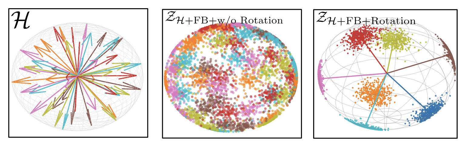
In it, different latent representations are used for RL tasks and RL dynamics
Using the dynamics latent h vector as a cluster center, and sampling task latent vectors z around it, one can obtain a clustered distribution of z vectors for different dynamics in task space
As shown in the figure below
The latent space here uses a normalized hypersphere, and a vMF distribution is used on the sphere as the sampling distribution for z
This note is a study note on the vMF distribution

From Gaussian Distribution to the vMF Distribution

Directional statistics studies data that lies on the unit sphere—compass readings, the direction of incident light, normalized word vectors, torsion angles of protein backbones, and so on. Such data cannot be modeled directly with an ordinary Gaussian, because the Gaussian is defined over the entire ${\mathbb{R}}^p$ . This article starts from the one-dimensional Gaussian and gradually transitions to the most central distribution in directional statistics: the von Mises–Fisher (vMF) distribution.

---

01 · One-Dimensional Gaussian Distribution

Let's start from the density function of a one-dimensional Gaussian distribution:

$$\begin{array}{}\text{(1.1)}& f(x)=\frac{1}{\sqrt{2\pi }\sigma }\exp (-\frac{(x-\mu {)}^2}{2{\sigma }^2})\end{array}$$

Expand the square in the exponent:

$$\begin{array}{}\text{(1.2)}& -\frac{(x-\mu {)}^2}{2{\sigma }^2}=\frac{\mu }{{\sigma }^2}x-\frac{x^2}{2{\sigma }^2}-\frac{{\mu }^2}{2{\sigma }^2}\end{array}$$

The last term is independent of $x$ and can be absorbed into the normalization constant. Thus, the "skeleton" of the Gaussian leaves only two parts: a linear term in $x$ , and a quadratic term.

$$\begin{array}{}\text{(1.3)}& f(x)\propto \exp (\frac{\mu }{{\sigma }^2}x-\frac{x^2}{2{\sigma }^2})\end{array}$$

The linear term ${\displaystyle \frac{\mu }{{\sigma }^2}}x$ determines the location of the distribution; the quadratic term $-{\displaystyle \frac{x^2}{2{\sigma }^2}}$ determines its shape. But on the sphere there is no place for a quadratic term — this is exactly why the vMF is simpler than the Gaussian.

One-Dimensional Gaussian (density curve + real-time sampling)

一维高斯分布

Drag the slider to observe how $\mu$ shifts the curve and $\sigma$ changes its width. The light-colored histogram is obtained by sampling from this distribution in real time, and it always matches the theoretical curve.

---

02 · Multivariate Isotropic Gaussian

Replace the scalar $x$ with a $p$ -dimensional vector $\mathbf{x}\in {\mathbb{R}}^p$ , and take the covariance to be isotropic ${\sigma }^2\mathbf{I}$ :

$$\begin{array}{}\text{(2.1)}& \mathcal{N}(\mathbf{x};\mathit{\mu },{\sigma }^2\mathbf{I})=(2\pi {\sigma }^2{)}^{-p/2}\exp (-\frac{\parallel \mathbf{x}-\mathit{\mu }{\parallel }^2}{2{\sigma }^2})\end{array}$$

Expand the squared Euclidean distance:

$$\begin{array}{}\text{(2.2)}& \parallel \mathbf{x}-\mathit{\mu }{\parallel }^2=\parallel \mathbf{x}{\parallel }^2-2{\mathit{\mu }}^{\mathrm{\top }}\mathbf{x}+\parallel \mathit{\mu }{\parallel }^2\end{array}$$

Substitute back into the exponential part:

$$\begin{array}{}\text{(2.3)}& -\frac{\parallel \mathbf{x}-\mathit{\mu }{\parallel }^2}{2{\sigma }^2}=\underset{\text{线性项}}{\underbrace{\frac{{\mathit{\mu }}^{\mathrm{\top }}\mathbf{x}}{{\sigma }^2}}}-\underset{\text{二次项}}{\underbrace{\frac{\parallel \mathbf{x}{\parallel }^2}{2{\sigma }^2}}}-\frac{\parallel \mathit{\mu }{\parallel }^2}{2{\sigma }^2}\end{array}$$

Thus the density can be written compactly as:

$$\begin{array}{}\text{(2.4)}& \mathcal{N}(\mathbf{x})\propto \exp (\frac{{\mathit{\mu }}^{\mathrm{\top }}\mathbf{x}}{{\sigma }^2}-\frac{\parallel \mathbf{x}{\parallel }^2}{2{\sigma }^2})\end{array}$$

KeyPoint

${\mathit{\mu }}^{\mathrm{\top }}\mathbf{x}$ measures the projection length of $\mathbf{x}$ along the mean direction. This term makes the density grow along the direction of $\mathit{\mu }$ ; while $-\parallel \mathbf{x}{\parallel }^2/(2{\sigma }^2)$ pulls the probability mass back toward the origin, preventing it from escaping to infinity.

---

03 · Normalizing the Distribution onto the Unit Sphere

Now impose the constraint: all data points lie on the unit sphere, i.e., $\mathbf{x}\in S^{p-1}$ , satisfying $\parallel \mathbf{x}\parallel =1$ .

Substituting $\parallel \mathbf{x}{\parallel }^2=1$ , that quadratic term immediately becomes a constant:

$$\begin{array}{}\text{(3.1)}& -\frac{\parallel \mathbf{x}{\parallel }^2}{2{\sigma }^2}=-\frac{1}{2{\sigma }^2}=\text{常数}\end{array}$$

The constant can be absorbed into the normalization factor. Thus only the linear term remains:

$$\begin{array}{}\text{(3.2)}& f(\mathbf{x})\propto \exp \left(\frac{{\mathit{\mu }}^{\mathrm{\top }}\mathbf{x}}{{\sigma }^2}\right)\end{array}$$

Decompose the mean vector into direction and magnitude: $\mathit{\mu }=\parallel \mathit{\mu }\parallel \cdot \hat{\mathit{\mu }}$ , where $\parallel \hat{\mathit{\mu }}\parallel =1$ . Then:

$$\begin{array}{}\text{(3.3)}& \frac{{\mathit{\mu }}^{\mathrm{\top }}\mathbf{x}}{{\sigma }^2}=\frac{\parallel \mathit{\mu }\parallel }{{\sigma }^2}{\hat{\mathit{\mu }}}^{\mathrm{\top }}\mathbf{x}=\kappa {\hat{\mathit{\mu }}}^{\mathrm{\top }}\mathbf{x}\end{array}$$

Physical meaning of the two parameters
$\kappa =\parallel \mathit{\mu }\parallel /{\sigma }^2$ is called the concentration parameter — the smaller the variance and the longer the mean, the more the distribution concentrates around $\hat{\mathit{\mu }}$ .
$\hat{\mathit{\mu }}$ is the mean direction, lying on the unit sphere.

At this point we have "guessed" the functional form of the vMF:

$$\begin{array}{}\text{(3.4)}& f(\mathbf{x})\propto \exp \left(\kappa {\mathit{\mu }}^{\mathrm{\top }}\mathbf{x}\right)\end{array}$$

Only one task remains: compute the normalization constant.

---

04 · The von Mises–Fisher Distribution

Let $\mathbf{x}\in S^{p-1}\subset {\mathbb{R}}^p$ , mean direction $\mathit{\mu }\in S^{p-1}$ , concentration $\kappa \ge 0$ :

$$\begin{array}{}\text{(4.1)}& f(\mathbf{x};\mathit{\mu },\kappa )=C_p(\kappa )\exp \left(\kappa {\mathit{\mu }}^{\mathrm{\top }}\mathbf{x}\right)\end{array}$$

The normalization constant is given by the modified Bessel function $I_{\nu }$ :

$$\begin{array}{}\text{(4.2)}& C_p(\kappa )=\frac{{\kappa }^{p/2-1}}{(2\pi {)}^{p/2}{I}_{p/2-1}(\kappa )}\end{array}$$

Why this form?

The core is computing this integral. Taking $\mathit{\mu }$ to point at the north pole, then ${\mathit{\mu }}^{\mathrm{\top }}\mathbf{x}=\cos \theta$ :

$$\begin{array}{}\text{(4.3)}& {\int }_{S^{p-1}}{e}^{\kappa {\mathit{\mu }}^{\mathrm{\top }}\mathbf{x}}d\sigma (\mathbf{x})={\mathrm{\Omega }}_{p-1}{\int }_0^{\pi }{e}^{\kappa \cos \theta }{\sin }^{p-2}\theta d\theta \end{array}$$

where ${\mathrm{\Omega }}_{p-1}=2{\pi }^{p/2}/\mathrm{\Gamma }(p/2)$ is the total surface area of the unit sphere. This integral has a closed-form solution:

$$\begin{array}{}\text{(4.4)}& {\int }_{S^{p-1}}{e}^{\kappa {\mathit{\mu }}^{\mathrm{\top }}\mathbf{x}}d\sigma (\mathbf{x})=(2\pi {)}^{p/2}{\kappa }^{1-p/2}{I}_{p/2-1}(\kappa )\end{array}$$

Taking the reciprocal gives $C_p(\kappa )$ . $◼$

The most common special case: $p=3$

The 3-dimensional sphere $S^2$ is the most common scenario in visualization and engineering. Using the elementary expressions for half-integer-order Bessel functions:

$$\begin{array}{}\text{(4.5)}& I_{1/2}(\kappa )=\sqrt{\frac{2}{\pi \kappa }}\sinh \kappa \end{array}$$

Substituting into $p=3$ :

$$\begin{array}{}\text{(4.6)}& C_3(\kappa )=\frac{{\kappa }^{1/2}}{(2\pi {)}^{3/2}{I}_{1/2}(\kappa )}=\frac{\kappa }{4\pi \sinh \kappa }\end{array}$$

Thus the vMF density on the 3-dimensional sphere is very clean:

$$\begin{array}{}\text{(4.7)}& f(\mathbf{x};\mathit{\mu },\kappa )=\frac{\kappa }{4\pi \sinh \kappa }\exp \left(\kappa {\mathit{\mu }}^{\mathrm{\top }}\mathbf{x}\right),\mathbf{x}\in S^2\end{array}$$

Limiting behavior
As $\kappa \to 0$ , $\sinh \kappa \approx \kappa$ , so $C_3\to 1/(4\pi )$ — exactly the uniform distribution on the sphere.
As $\kappa \to \mathrm{\infty }$ , the density collapses to a Dirac $\delta$ function located at $\mathit{\mu }$ .

The vMF distribution on $S^2$

S² 上的 vMF 分布

Particles on the sphere below follow $\mathrm{vMF}(\mathit{\mu },\kappa )$ . Drag the sphere to rotate the view; increase $\kappa$ to observe how the particles converge from a uniform spread into a spherical cap; change ${\theta }_{\mu },{\varphi }_{\mu }$ to observe how the entire cap migrates.

05 · Projecting a Normal Distribution onto the Sphere

We now know the definitions of the Gaussian and vMF distributions. So how exactly are they connected?

The answer: normalize Gaussian samples to unit length. Let $\mathbf{y}\sim \mathcal{N}(\mathit{\mu },{\sigma }^2\mathbf{I})$ be a Gaussian vector in ${\mathbb{R}}^p$ , and set

$$\begin{array}{}\text{(5.1)}& \mathbf{x}=\frac{\mathbf{y}}{\parallel \mathbf{y}\parallel }\in S^{p-1}\end{array}$$

Then the distribution followed by $\mathbf{x}$ is called the projected normal distribution, whose density is:

$$\begin{array}{}\text{(5.2)}& f(\mathbf{x};\mathit{\mu },{\sigma }^2)\propto {\int }_0^{\mathrm{\infty }}{r}^{p-1}\exp (-\frac{\parallel r\mathbf{x}-\mathit{\mu }{\parallel }^2}{2{\sigma }^2})dr\end{array}$$

Expanding the norm, the dependence on $r$ becomes clear:

$$\begin{array}{}\text{(5.3)}& \parallel r\mathbf{x}-\mathit{\mu }{\parallel }^2=r^2-2r({\mathit{\mu }}^{\mathrm{\top }}\mathbf{x})+\parallel \mathit{\mu }{\parallel }^2\end{array}$$

In the isotropic case (covariance ${\sigma }^2\mathbf{I}$ ), after integrating over $r$ , all parts involving $\mathbf{x}$ reduce to just $\exp (\parallel \mathit{\mu }\parallel {\hat{\mathit{\mu }}}^{\mathrm{\top }}\mathbf{x}/{\sigma }^2)$ . Thus:

$$\begin{array}{}\text{(5.4)}& f(\mathbf{x};\mathit{\mu },{\sigma }^2)=f_{\mathrm{vMF}}(\mathbf{x};\hat{\mathit{\mu }},\kappa ),\kappa =\frac{\parallel \mathit{\mu }\parallel }{{\sigma }^2}\end{array}$$

Core conclusion
Radially normalizing an isotropic Gaussian yields exactly the vMF distribution. Conversely, vMF can also be viewed as "an isotropic Gaussian defined on the sphere." Two seemingly unrelated distributions differ only by a single normalization.

Geometric intuition

Imagine a Gaussian cloud in ${\mathbb{R}}^3$ centered at $\mathit{\mu }$ . Now slide each point along the ray from the origin onto the unit sphere — direction unchanged, only the radius changes. The cloud originally scattered in space gets "smeared" onto the sphere, forming a concentrated spot in the direction of $\mathit{\mu }$ .

The thinner the cloud (smaller $\sigma$ ) and the farther the center is from the origin (larger $\parallel \mathit{\mu }\parallel$ ), the more compact the spot — this is exactly what $\kappa =\parallel \mathit{\mu }\parallel /{\sigma }^2$ means.

Continuous transition from Gaussian to vMF

高斯 → vMF 的连续过渡

The initial state ( $t=0$ ) is an isotropic Gaussian cloud in ${\mathbb{R}}^3$ , shown in amber; drag the transition slider or enable autoplay, and the particles slide radially onto the sphere ( $t=1$ ), with the color gradually turning cyan — that is the vMF distribution.

Drag the $\sigma$ slider to change the Gaussian's spread, thereby changing the final vMF's $\kappa$ . Observe: the smaller $\sigma$ is, the more concentrated the final spot on the sphere.

---

06 · Sampling: Wood's Algorithm

To generate points on the sphere following a vMF distribution, the key is to exploit rotational invariance: first sample along the $z$ axis, then rotate the result to $\mathit{\mu }$ .

Step 1: Sample the polar angle cosine $\omega =\cos \theta$

On $S^2$ , the marginal density of $\omega$ is proportional to $e^{\kappa \omega }$ (the $\sin \theta$ factor in the area element cancels out exactly when $p=3$ ). The cumulative distribution function is:

$$\begin{array}{}\text{(6.1)}& F(\omega )=\frac{e^{\kappa \omega }-e^{-\kappa }}{e^{\kappa }-e^{-\kappa }}\end{array}$$

Let $F(\omega )=u$ , $u\sim U(0,1)$ , and solve for the inverse:

$$\begin{array}{}\text{(6.2)}& \omega =1+\frac{1}{\kappa }\ln (u+(1-u)e^{-2\kappa })\end{array}$$

Numerical stability
When $\kappa$ is large, computing $e^{2\kappa }$ directly will overflow. The expression above rewrites the exponential as $e^{-2\kappa }$ , which automatically degenerates to $\omega \approx 1+\ln (u)/\kappa$ when $\kappa \to \mathrm{\infty }$ , with no overflow throughout.

Step 2: Sample the azimuth and assemble

Take $\phi \sim U(0,2\pi )$ , let $s=\sqrt{1-{\omega }^2}$ :

$$\begin{array}{}\text{(6.3)}& {\mathbf{x}}_0=(s\cos \phi ,s\sin \phi ,\omega )\end{array}$$

Step 3: Rotate to $\mathit{\mu }$

Construct an orthonormal basis $({\mathbf{e}}_1,{\mathbf{e}}_2,\mathit{\mu })$ with $\mathit{\mu }$ as the third axis, and output:

$$\begin{array}{}\text{(6.4)}& \mathbf{x}=x_{0,1}{\mathbf{e}}_1+x_{0,2}{\mathbf{e}}_2+x_{0,3}\mathit{\mu }\end{array}$$

---

07 · Key Properties and Estimation

Mean Resultant Vector Length

The expectation of the vMF has a very concise form—the direction is simply $\mathit{\mu }$ , and the length depends only on $\kappa$ :

$$\begin{array}{}\text{(7.1)}& \mathbb{E}[\mathbf{x}]=A_p(\kappa )\mathit{\mu },A_p(\kappa )=\frac{I_{p/2}(\kappa )}{I_{p/2-1}(\kappa )}\end{array}$$

When $p=3$ , it reduces to the Langevin function form you may have seen before:

$$\begin{array}{}\text{(7.2)}& A_3(\kappa )=\coth \kappa -\frac{1}{\kappa }\end{array}$$

It grows monotonically from $0$ to $1$ : at $\kappa =0$ the direction is completely random, and at $\kappa \to \mathrm{\infty }$ all points point toward $\mathit{\mu }$ .

Parameter Summary

Parameter	Value	Meaning
$\mathit{\mu }$	$S^{p-1}$	mean direction, unit vector
$\kappa$	$[0,\mathrm{\infty })$	concentration; larger means more concentrated
$\kappa =0$	—	uniform distribution on the sphere
$\kappa \to \mathrm{\infty }$	—	degenerates to the point $\mathit{\mu }$
$p=2$	—	circular vM distribution, $C_2=1/(2\pi I_0(\kappa ))$
$p=3$	—	$C_3=\kappa /(4\pi \sinh \kappa )$

Maximum Likelihood Estimation

Given samples $\{{\mathbf{x}}_1,\dots ,{\mathbf{x}}_n\}$ , the log-likelihood is:

$$\begin{array}{}\text{(7.3)}& \ell (\mathit{\mu },\kappa )=n\ln C_p(\kappa )+\kappa {\mathit{\mu }}^{\mathrm{\top }}\left(\sum _{i=1}^n{\mathbf{x}}_i\right)\end{array}$$

Differentiating with respect to $\mathit{\mu }$ immediately yields: $\hat{\mathit{\mu }}$ is the direction of the sample resultant vector, i.e.

$$\begin{array}{}\text{(7.4)}& \hat{\mathit{\mu }}=\frac{\sum _i{\mathbf{x}}_i}{\Vert \sum _i{\mathbf{x}}_i\Vert }\end{array}$$

And $\kappa$ is implicitly determined by the equation $A_p(\hat{\kappa })=\parallel \sum {\mathbf{x}}_i\parallel /n$ —there is no closed-form solution, so numerical solving is required (Newton's method typically converges within a few iterations).

---

08 · Summary

$$\begin{array}{rl}& \text{各向同性高斯}\mathcal{N}(\mathbf{x};\mathit{\mu },{\sigma }^2\mathbf{I})\\ & \to \text{展开指数}\\ & \to \text{施加约束}\parallel \mathbf{x}\parallel =1\\ & \to \text{二次项变成常数}\\ & \to \text{只剩}\exp (\kappa {\mathit{\mu }}^{\mathrm{\top }}\mathbf{x})\\ & \to \text{补上球面归一化常数}\\ & \to \mathbf{\text{vMF 分布}}\end{array}$$

The isotropic Gaussian (projected normal) on the sphere and the vMF are equivalent. Because for points on the sphere, $\parallel \mathbf{x}{\parallel }^2=1$ in the Gaussian density is a constant; the quadratic form ${\mathbf{x}}^{\mathrm{\top }}{\mathrm{\Sigma }}^{-1}\mathbf{x}$ of the projected normal also degenerates to a constant when $\mathrm{\Sigma }={\sigma }^2\mathbf{I}$ . The two give exactly the same distribution family.

This also explains why the vMF is the undisputed "Gaussian" of directional statistics: it is simple, unimodal, has a conjugate prior, has efficient sampling algorithms, and at the two extremes of $\kappa$ it covers the uniform distribution and a deterministic direction, respectively.

contents

1. From Gaussian Distribution to the vMF Distribution
   1. 01 · One-Dimensional Gaussian Distribution
      1. One-Dimensional Gaussian (density curve + real-time sampling)
   2. 02 · Multivariate Isotropic Gaussian
      1. KeyPoint
   3. 03 · Normalizing the Distribution onto the Unit Sphere
   4. 04 · The von Mises–Fisher Distribution
      1. Why this form?
      2. The most common special case: p=3
      3. The vMF distribution on S2
   5. 05 · Projecting a Normal Distribution onto the Sphere
      1. Geometric intuition
      2. Continuous transition from Gaussian to vMF
   6. 06 · Sampling: Wood's Algorithm
      1. Step 1: Sample the polar angle cosine ω=cos⁡θ
      2. Step 2: Sample the azimuth and assemble
      3. Step 3: Rotate to μ
   7. 07 · Key Properties and Estimation
      1. Mean Resultant Vector Length
      2. Parameter Summary
      3. Maximum Likelihood Estimation
   8. 08 · Summary